Fantasy sports platform Sleeper has developed an API to give players access to a trove of league-specific data that is not publicly accessible on other platforms. Things like like historical roster makeup, results over time, and setting changes are now easily viewable by anyone who plays fantasy on Sleeper. Needless to say, the Sleeper API represents a perfect opportunity to build and share a user-friendly, Excel based tool.
Most Fantasy Football leagues operate under slightly different sets of rules. In the league I run, we’ve implemented some unique payouts during our regular season. The top two scorers each week get $5, and everyone who wins a regular season match gets $4. As commissioner, one of my duties is to track these payouts over the course of the season so that each player gets the correct amount at the end of the year. This used to be a task that I loathed with a fiery passion!
When we started these payouts I had to manually enter scores from our league into a spreadsheet to calculate the correct amounts. This annoying process often led to mistakes and miscalculations. Thankfully those days are over now that I have the Hyzermetrics Fantasy Football Payout Tracker!
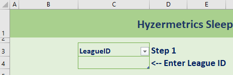
The tracker gives commissioners the ability to track custom payout structures in their league. It relies on the LeagueID, which is can be found on your browser any time you access your league.
Once you have your LeagueID, enter it into cell C4 of the tracker.
Next, populate your payouts! You can have a prize for a weekly win, and you can assign prizes for each position.
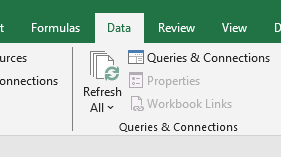
Finally, go up to the Data ribbon and click Refresh All. The first time you do this, you may see a pop-up about privacy levels. In this case, you can check the “Ignore Privacy Levels” checkbox.
Congrats, once you’ve gone through these steps you will now have a functioning payout calculator! Refresh it each week to update the payout amounts. Hopefully this tool will save my fellow commissioners a headache or two this Fantasy Football season.
A few months ago I decided to combat my usual winter descent into laziness by purchasing an exercise bike. Naturally, with this big purchase came my desire to use data to track my progress throughout the winter. Namely:
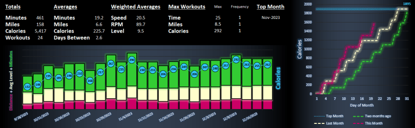
How do my recent workouts compare to my past workouts?
What are my records on the bike?
Am I doing better so far this month than last month? How about the month before?
Introducing the Hyzermetrics Workout Dashboard! The dashboard lets users visualize workout trends on the Nautilus U616 using the bike’s export to USB feature. Follow the below steps to begin using the dashboard.
Create a folder on your desktop called WorkoutArchive
Download the SAMPLE DATA file and save as .csv into the newly created folder (WordPress wouldn’t let me upload a .csv, so I had to upload as .xlsx)
Download the MyWorkouts spreadsheet and save it to your desktop
Follow the instructions on the MyWorkouts spreadsheet to track your progress!
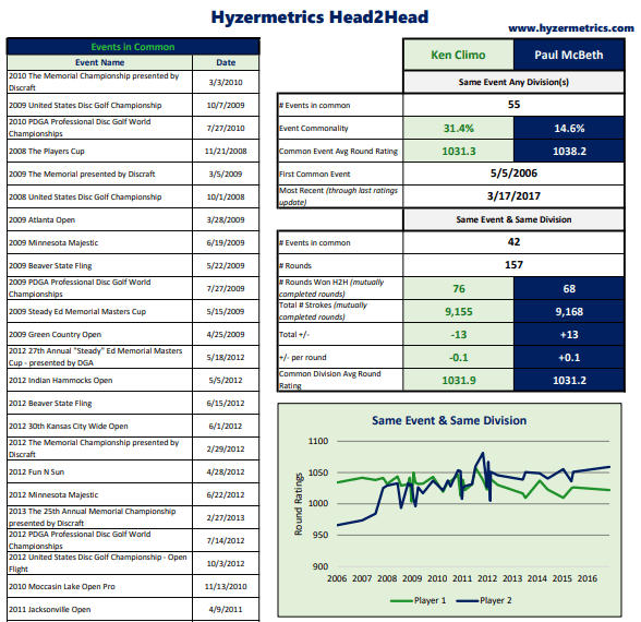
The disc golf careers of legends Ken Climo and Paul McBeth overlapped for over a decade. In the mid-2010s, As Ken Climo began playing fewer tournaments, and even fewer in the MPO division, McBeth’s domination began. Although we won’t ever get to see these two athletes compete head-to-head in their primes, they did compete against one another at 42 tournaments, encompassing 157 rounds from 2006 to 2017. That’s a lot of disc golf tournaments featuring two of the best the sport has ever seen! With such a large sample size, we would usually expect one of the two players to emerge as the clear victor in their head-to-head matchups. Somehow, that didn’t happen with Climo and McBeth. The difference in their total throw counts across these events: a mere thirteen strokes!
For the first time ever, disc golfers now have access to data that gives cool head-to-head stats like the one above. Introducing the Hyzermetrics Head2Head spreadsheet! It gives a disc golfers and fans the opportunity to compare head-to-head stats of any two current PDGA members, all you need are PDGA numbers! The Hyzermetrics Head2Head spreadsheet allows disc golfers to: · Quickly get cool stats from head-to-head matchups between disc golf’s best – Pick your favorite disc golfers and give it a shot! · Figure out which tournaments they’ve played with specific people – how many times have you asked yourself “where have I played with that person before…?” The Hyzermetrics will list every tournament you’ve played with the other person and how you’ve done in those tournaments · Earn serious bragging rights with friends – regularly remind your buddy that you’ve shot better in 70% of the events you’ve played together… or if that percentage doesn’t work out in your favor maybe keep that on the DL.
In the Climo vs Mcbeth example from earlier, Hyzermetrics Head2Head shows how the matchups between the champs changed over the years. It makes sense that 54 year-old Climo dominated the first three years of the battle (2006-2009) as 32 year-old McBeth came onto the scene. The next three years saw a back-and-forth struggle between the two powerhouses. As McBeth established dominance in the disc golf world in 2012 he slowly started to make up the ground he’d lost in the early years of the matchup.
The decade-long head-to-head battle between Ken Climo and Paul McBeth likely came to an end in 2017, with Climo playing few PDGA tournaments, and even fewer in the MPO division. While I am not prepared to weigh in on which disc golfer is the greatest of all-time, Hyzermetrics Head2Head can tell us how these incredible athletes fared when they competed against one-another.
NOTE: When you first open Hyzermetrics Head2Head you will need to enable External Data connections. You also may get a popup about Privacy Levels. If you do, check the “Ignore Privacy Levels” box and in the dropdowns on the right-hand side set both options to Public
As hinted in my last post, the ability to systematically match PDGA Events with their corresponding Event Numbers has a number of implications that can help disc golfers make sense of the ever-growing amount of data available on the web. The Hyzermetrics Eventfinder is the first of many applications of the PDGA Event Number Database, and I couldn’t be more excited to share!
Fortunately for disc golfers, the PDGA website has always had a pretty good search feature that has more or less stood the test of time. But the Hyzermetrics Eventfinder provides users with a handful of search datapoints that the PDGA Website does not:
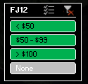
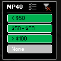
1. Search by Division – The Hyzermetrics Eventfinder can help you quickly weed out events that don’t offer your division(s) of interest. For example, suppose you play MP40, but would like to find a tournament that you and your daughter (FJ12) can both play. Many tournaments do not offer both of these divisions, and until now there has not been a way to easily identify those that do. The Eventfinder will help. Filter on each of the divisions of interest (tip: hold CTRL to select multiple buttons within a single slicer box) and you will be left only with the tournaments that offer MP40 and FJ12.
2. Search by Entry Fee – Money is tight these days, but the Hyzermetrics Eventfinder can help disc golfers find events that fit their budget. Don’t want to break the bank to play a sanctioned event? Pick a <$50 filter in your division of choice to weed out the events that are out of your budget.
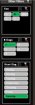
3. Search by Number of Days and Starting Day of Week – Weekend warriors know that time can be fleeting. The Hyzermetrics Eventfinder can help these golfers find tournaments that fit into their busy schedules. If you’re looking for a B-Tier but can only play on Saturdays, set the below filters and you will see only the events that meet these criteria!
A few notes about the Hyzermetrics Eventfinder:
You can update the data yourself! That’s right, once you download the Hyzermetrics Eventfinder, you do not need to re-download it to get the latest and greatest event listing. Simply click CTRL+ALT+F5 to refresh the tournament list.
It only contains events that appear on the PDGA calendar
It only contains events that take registration through discgolfscene.com
It does NOT contain any X-tier or League Sanctioned events
This new tool, while useful, is just the tip of the iceberg of what we can do when we can match PDGA Events with their Event Numbers.
PDGA Event Numbers are rarely of importance to most disc golfers. But for data enthusiasts, they are a piece of the puzzle that can link data from a disc golfer’s PDGA page to data from the events they play. Unfortunately, PDGA Event Number listings have not historically been available. Until now. Hyzermetrics is excited to introduce the PDGA Event Number Database! This Database will be refreshed on this post on a monthly basis. No crazy macros, no complicated analysis, just a simple Excel spreadsheet for you to use in your own data exploration.
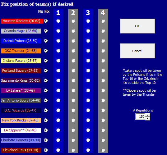
Alrighty folks, we are a mere 20 minutes away from the start of ESPN’s 2022 NBA Draft Lottery Coverage! I’m going to kick the night off by running a simulation of 150 trials from the Hyzermetrics NBA Draft Lottery Simulator. For this initial run, I won’t be fixing any draft positions or anything, just going to change the number of repetitions and let it ride. I’ll be back with the results shortly.
7:56 PM ET
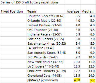
Alright, the results of our set of 150 trials are in. As expected, the Rockets, Magic, Pistons, and Thunder finished with the highest average and median draft positions. Nothing too crazy here. What I would like to focus on is our famous p(max)/p(observed) likelihood ratio stat that I’ve talked about at length in past articles. For the series of 150 repetitions that we just ran, the average ratio was 45.8, which seems relatively high, but check out the median… it’s only 5.7. This means that half of the random trial reps we just ran came in with a max:observed likelihood ratio at or under 5.7. As we go through the lottery, this median number is important to note, as we can benchmark the likelihood ratio that we’re about to observe against this unadulterated 5.7 median in our initial set of trials.
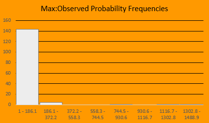
Median likelihood ratio of 5.7 will be used to benchmark the actual result at the end of the lottery143 of the 150 reps ended with p(max)/p(observed) less than 186.1…
8:07 PM ET
Doing a little digging into the numbers from our initial set of trials. There were some really unlikely outcomes that brought the average likelihood ratio way up! In fact 132 of the 150 trials had a max:observed likelihood ratio under the average of 45.8. Based on this, I’d be relatively surprised if the observed result of the NBA Draft Lottery has a ratio greater than the median of 5.7, and I’d be downright shocked if it we see an outcome with a ratio that exceeds 45.8.
8:13 PM ET
Ok, ESPN let’s announce the results already.
8:21 PM ET
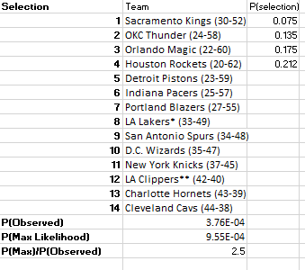
Alright, we are pretty much locked to get a very chalk-y result here. We know that the Kings are picking in the top 4… the least likely result remaining is 1) Kings, 2) Thunder, 3) Magic, 4) Rockets. Let’s see what that result would look like from a probability perspective…
This result, which is the least likely outcome we could observe given the remaining four teams, would have a likelihood ratio of 2.5
8:30 PM ET
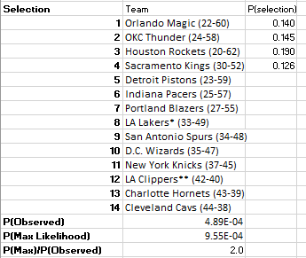
The results are in! The first four picks in the 2022 NBA Draft will be:
Orlando Magic
OKC Thunder
Houston Rockets
Sacramento Kings
Let’s run another simulation with this result built in as fixed:
With p(max)/p(observed) roughly equal to 2, the actual result of the 2022 NBA Draft Lottery was about half as likely to occur than the most likely outcome. Based on our initial series of trials, this result is rather unremarkable, however there are two important observations we made in the Draft Lottery that were unlikely:
The Kings got a top 4 pick
The Rockets draft after the OKC Thunder
To conclude the evening, I am already preparing the enhancements for next year’s NBA Draft Lottery, can’t wait to share them with you! Thanks for joining for the first Hyzermetrics Live NBA Draft Lottery Simulation!
The day we’ve all been waiting for is finally here! That’s right, we are just one week away from the 2022 NBA Draft Lottery! And fortunately, Hyzermetrics has just the tool to help you and your crew commemorate the occasion.
If you need a refresher on the mechanics of the NBA Draft Lottery, don’t worry, we’ve got you covered. Here’s how it works:
“The 38th annual NBA Draft Lottery will determine the order of selection for the first 14 picks of the 2022 NBA Draft. Drawings will be conducted to determine the first four picks in the NBA Draft. The remainder of the lottery teams will select in positions five through 14 in inverse order of their 2021-22 regular-season records…
Fourteen ping-pong balls numbered 1 through 14 will be placed in a lottery machine. There are 1,001 possible combinations when four balls are drawn out of 14, without regard to their order of selection. Before the lottery, 1,000 of those 1,001 combinations will be assigned to the 14 participating lottery teams…
The Draft selections for the remainder of the first round (No. 15-30) and the entire second round (No. 30-60), are determined by reverse order of regular season record. Each NBA team gets one selection in the first round and one selection in the second round.”
The first tidbit to note is that at first glance, the NBA Draft Lottery is set up a little bit differently than the Hyzermetrics Fantasy Draft Lottery Simulator. That said, we can actually re-configure the Hyzermetrics Fantasy Draft Lottery to match this procedure… instead of assigning ball numbers to Lottery participants, we assign “combination numbers” to each participant and pull four combination numbers out of the Hyzermetrics Lottery Machine. Here’s what this year’s set up will be:
Team
# Combinations
Min Combo Num
Max Combo Num
Houston Rockets (20-62)
140
1
140
Orlando Magic (22-60)
140
141
280
Detroit Pistons (23-59)
140
281
420
OKC Thunder (24-58)
125
421
545
Indiana Pacers (25-57)
105
546
650
Portland Blazers (27-55)
90
651
740
Sacramento Kings (30-52)
75
741
815
LA Lakers* (33-49)
60
816
875
San Antonio Spurs (34-48)
45
876
920
D.C. Wizards (35-47)
30
921
950
New York Knicks (37-45)
20
951
970
LA Clippers** (42-40)
15
971
985
Charlotte Hornets (43-39)
10
986
995
Cleveland Cavs (44-38)
5
996
1000
Before we dive in, there are some really great articles and resources on the subject of the NBA Draft Lottery, and even a cool web-based simulator that you should check out. Once you’re done with those, you will not want to miss the cool features in the Excel based Draft Lotto Simulator to take your knowledge of the NBA Draft Lottery to the next level.
Lotto Simulator: 2022 NBA Draft Lottery Edition
To recap, here are some high level facts about the NBA Draft Lottery:
The 14 teams that did not make the playoffs participate in the Draft Lottery
14 ping-pong balls numbered 1-14 are placed into the lottery machine
To determine the first pick, four ping-pong balls are chosen. The (non-ordered) combination of numbers drawn represents the winning combination.
Example of a winning combination might be: 6, 13, 10, 3. Whichever team has this combination assigned to them will get the first pick
To determine picks 2-4, the same process as above is performed, discarding any combinations of teams that have already been drawn
Picks 5-14 are determined in reverse Regular Season Standings order.
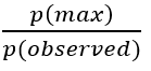
This ratio gives us an idea of just how unusual an observation in a particular lottery is. It tells us precisely how many times more likely we are to see the maximum likelihood outcome of a given lottery than we are to see a particular observation. Once we have this ratio, we can then compare this result to other lottery results to see which ones were more or less likely to occur. As an example If the ratio is equal to 2.0, then the max likelihood outcome is two times as likely to occur than the observed outcome. The minimum possible p(max)/p(observed) ratio is 1.0.
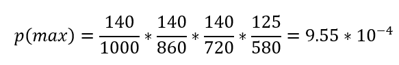
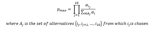
For the NBA Draft Lottery p(max) is calculated as follows:
Note that there are actually six different outcomes that have this probability. The outcomes that share this probability are:
Rockets, Magic, Pistons, Thunder
Magic, Rockets, Pistons, Thunder
Pistons, Rockets, Magic, Thunder
Magic, Pistons, Rockets, Thunder
Rockets, Pistons, Magic, Thunder
Pistons, Magic, Rockets, Thunder
The NBA Draft Lottery Simulator is fully prepared to help you analyze the lottery trials you run. Here’s what you can do with it:
Run a simple NBA Draft Lottery simulation and tell you the Max:Outcome likelihood ratio for the trial
Run a series of up to 150 Draft Lottery simulations and show you statistics describing the trials
Fix the draft location of one or more teams to see how probabilities and selections are impacted
Let’s run through some examples!
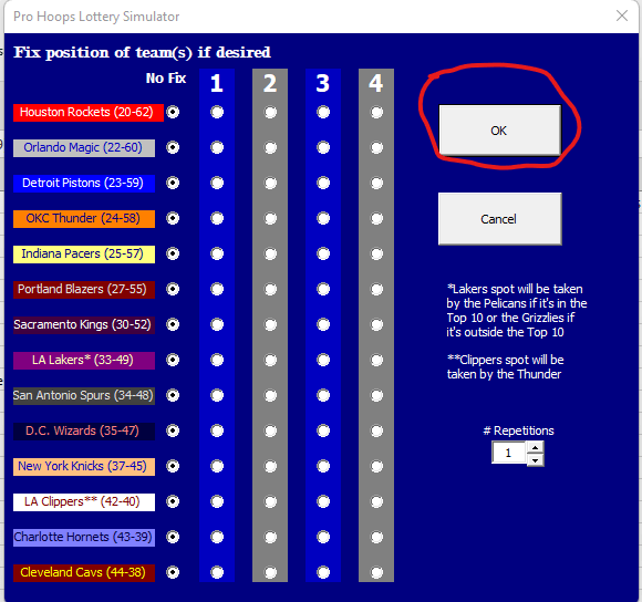
Run a simple Draft Lottery
Click on the blue NBA Draft Lottery button
Press OK
View the results of the trail. In the trial screenshotted below, the outcome was fairly chalky… the Thunder got the first pick, then the top likelihood teams got each of the next three picks for a p(max)/p(observed) of 1.6
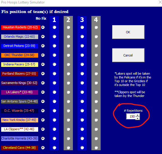
Run a series of up to 150 Draft Lottery simulations and show you statistics describing the trials
Click on the blue NBA Draft Lottery button
Select the desired number of repetitions
Press OK
The simulator will run the specified number of simulations and create a new sheet to tell you all about the results! Here are some stats about the simulation we just ran:
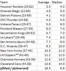
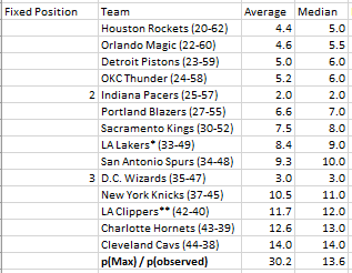
In this series of 150 trials, we can see that the Magic had an average draft position of 4.0 and a median draft position of 5.0.
Average p(max)/p(observed) was 18.3, while the median 6.8
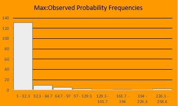
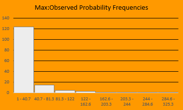
131 of the 150 trials had a p(max)/p(observed) between 1 and 32.3
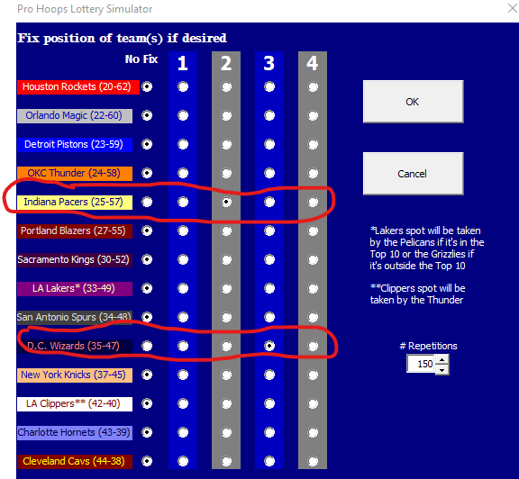
Fix the draft location of one or more teams to see how probabilities and selections are impacted
Click on the blue NBA Draft Lottery button
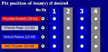
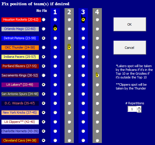
Select the draft positions of the teams you’re interested in fixing for the simulation. In this experiment, I am looking to run a simulation of outcomes when the Pacers get selected to pick 2nd AND the Wizards get selected to pick 3rd.
Select the desired number of repetitions
Press OK
The simulator will run the specifiednumber of simulations and create a new sheet to tell you about the results… but wait… The teams you chose are fixed in the draft positions you selected! Under the conditions I specified in step 2, we can see that both the average and median of p(max)/p(observed) is much higher than when we didn’t specify any conditions. The whackier the conditions, the higher these ratios will be!
Try out the Simulator for yourself, and stay tuned to Hyzermetrics on May 17th as we Live Simulate the NBA Draft Lottery in real-time!
A couple years ago, my Fantasy Football league passed a rule that said our draft order would be determined by lottery each year. As commissioner, it was my job to implement this rule. My initial idea was to buy an actual full-blown lottery ball machine. How cool would that be?! But due a combination of frugality and laziness, I never actually ended up buying one. I also debated using the tried-and-true “numbers out of a hat” method. It was simple and would get the job done, but I decided that I wanted to create something with a little flair.
Enter the Lotto Simulator. This spreadsheet has the ability to run a couple different types of lotteries, and the fun part, as always, is in the math! Now, there’s a whole lot of interesting math we can do for lotteries like this, and maybe I’ll do a super deep dive in a future post. But today, I’ll focus only on what I automated in the Lotto Simulator spreadsheet, just please know that this is only scratching the surface!
Draft lotteries can be set up in a couple different ways. For our Fantasy Football league, we set it up as follows:
Each team is assigned between 1 and 10 lottery balls based on their finish in the previous regular season
5th place – 10 balls
6th place – 9 balls
7th – 8 balls
8th – 7 balls
9th – 6 balls
10th – 5 balls
4th – 4
3rd – 3
2nd – 2
1st – 1
When someone’s lottery ball is selected, they get to pick their draft position
What is the most likely outcome of our league’s draft lottery, and what is the probability of that happening?
The most likely outcome is that for each draw, the event with the highest probability occurs. Based on the Plackett-Luce model, doing this ten times gives us:
Given our league’s lottery setup:
After identifying the probability of the max likelihood outcome above, suppose we run a lottery that yields the below selection order:
7th place – 8 balls
8th place – 7 balls
6th place – 9 balls
5th place – 10 balls
2nd place – 2 balls
9th place – 6 balls
10th place – 5 balls
1st place – 1 ball
4th place – 4 balls
3rd place – 3 balls
It’s reasonable to ask “What was the probability of the observed result?” The lotto spreadsheet gives us the answers to this question!
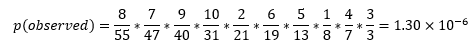
The probability of observing our result is:
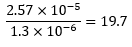
Unfortunately, this number doesn’t tell us much on its own. It’s a tiny number, but so too is our max likelihood number we derived earlier. How do we make sense of it all? The p(Max)/p(Observed) ratio is our answer! This number tells us how many times more likely we are to see the max likelihood outcome than the observed outcome for a given lottery. In the example of my league, this ratio is equal to:
This means that we are 19.7 times more likely to observe the max likelihood result than the result we observed.
Let’s do the same lottery again. Suppose that our second lottery gives these results:
7th place – 8 balls
5th place – 10 balls
9th place – 6 balls
4th place – 4 balls
10th place – 5 balls
6th place – 9 balls
3rd place – 3 balls
8th place – 7 balls
2nd place – 2 balls
1st place – 1 ball
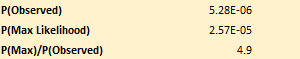
From this lottery, our p(max)/p(observed) ratio is 4.9…. so we can say that the result of the second lottery was a far more likely outcome than the result of the first!
And there we have it. The Lotto Simulator spreadsheet not only runs a lottery, but it also gives us a surface level understanding of the results we observe. Now, when your league-mates complain that a lottery is “rigged,” you can use the Lotto spreadsheet to see just how unusual the results of your lottery are.
Here’s what to do:
Download the Lotto Simulator spreadsheet
You many need to click “Enable Content” to enable macros
Choose the type of lottery you want to run
In addition to the Draft Lottery discussed in this article, the spreadsheet also has a built in Traditional Lottery option. Try it out!
Run the Lotto Simulator spreadsheet for any and all of your lottery needs!
In my most recent post I introduced a process to estimate the probability of me making a putt in my garage. I also provided a tool for others to do the same (though one doesn’t necessarily need to be in their garage if the weather cooperates). In that exercise, I assumed that each putt had an equal probability of success, and the number of putts made in a series of fifty attempts could be represented by random variable with a Binomial probability distribution.
Shifting gears, suppose that instead of garage putts, we instead perform a different series of tests:
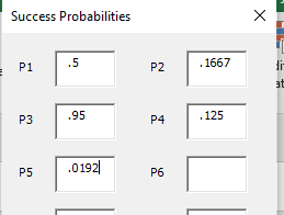
Flip a coin, success if heads p(success) = .5
Roll a six-sided die, success if a six is rolled p(success) = .1667
Go out to my garage and make a putt that has a 95% success probability p(success)= .95
Roll an eight-sided die, success if an eight is rolled p(success) = .125
Correctly guess a card pulled at random from a standard deck of 52 cards p(success) = .0192
With this series of tests, we can ask “what is the probability that we’ll see x successes?” But sadly, our beloved Binomial distribution is not sufficient to answer this question.
Before we deep-dive into the solution, let’s eyeball this series of tests and see if we can make any guesses as to what the outcome is likely to be. It seems like it would be extremely unlikely to see less than one success in this series of tests, because one trial in the bunch, the 95% garage putt, has a very high probability of success. The probability of missing that putt AND missing all the others would seem pretty low. But other than the putt and the coin flip, all the other tests seem like they’re pretty unlikely to hit, so it seems like we probably won’t see three or more successes.
If we let K = the # of successes in our weird series of trials, then K takes on a Poisson Binomial Distribution, which is similar to the Binomial Distribution except the probability of success varies with each trial. If we wanted to see the probability of observing exactly three successes, we would need to analyze the probability of each possible outcome that contains three successes and add their probabilities. If we denote 1 as a success and 0 as a failure, then we can use the below chart to identify P(K = 3)
Every possible outcome that contains exactly three successes
Adding these up gives us the probability of observing exactly three successes in our series of trials:
As you can see, the math for finding the p(K = k) for a Poisson Binomial random variable can be fairly tedious, especially as the number of trials increases. In fact, for n trials, the number of different outcomes that need to be individually analyzed is equal to 2n and for any number of successes k:
where Fk is the subset of all subsets of k integers that can be selected from n trials and Ac is the complement of A.
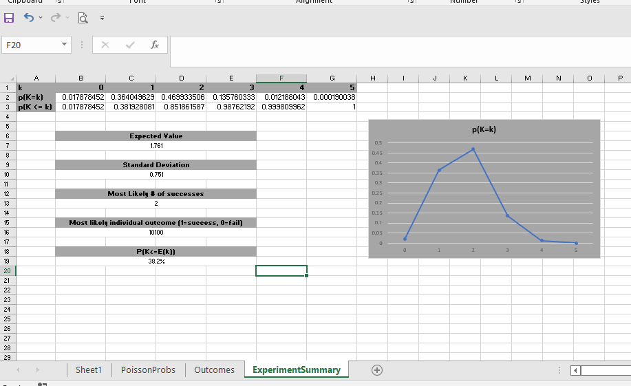
For more than a couple trials, the arithmetic can amount to quite a lot of work! There are a number of fancy stats software programs out there that might be able to help, but fortunately I’ve developed a way to do it in Excel! In the Poisson Binomial – Fantasy Football Strength of Schedule worksheet, you can run a Poisson Binomial analysis for a set of up to 20 trials! Let’s use it for our series of tests discussed earlier.
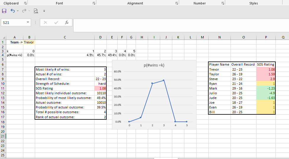
In seconds, the worksheet shows exactly how many successes I can expect to have along with probabilities for each possible number of successes. As we discussed earlier when we were just eyeballing the set of tests, the probability of observing k=0 successes is very low, less than 2%. But it is even more unlikely for us to observe k>=4 successes! The number of successes we are most likely to observe in this series of tests is 2.
We now have a way to run a quick analysis of a Poisson Binomial Distributed random variable in MS Excel! Try it out for yourself, then let’s explore an application.
Application: Fantasy Football Strength of Schedule
How many times has your fantasy football team had a fantastic week only to suffer a loss to the only team in the league with more points than you? Conversely, have you ever been pleasantly surprised as you skate through the season with mediocre performances that happen to come against teams that do even worse? Until now, it was difficult to quantify and compare exactly how lucky or unlucky fantasy players were over the course of a season.
Suppose that we were to hide the weekly matchups in your fantasy football league and instead we only saw each team’s point totals each week. We’d be able to get a pretty good idea of how many wins each league participant should have throughout the season, then we could compare that number to the number of wins they actually have. Using this comparison, we can determine if a fantasy team has had a hard schedule or an easy one.
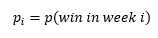
The probability that a team will win their fantasy football match in a given week is a function of the rank of their score in that week. If a team finishes first in points in a given week, then they’re guaranteed to win, no matter who the schedule has them playing against that week. If they finish last in points for the week, then no amount of good fortune will save them, and they will lose. A team that finishes second in points during a given week is probably going to win, but there’s a small chance the schedule has them matched up against the team that finishes first, in which case they will suffer an unfortunate loss! In general, the probability of a win can be expressed as follows:
If we do this over the course of the season of n weeks, we can generate set of probabilities that we can use in a Poisson Binomial analysis with:This analysis tells us the exact probability that each team will win any number of games throughout the year. We can then compare these probabilities against the number of wins each team ACTUALLY has. This tells us who which teams are lucky and which ones aren’t.
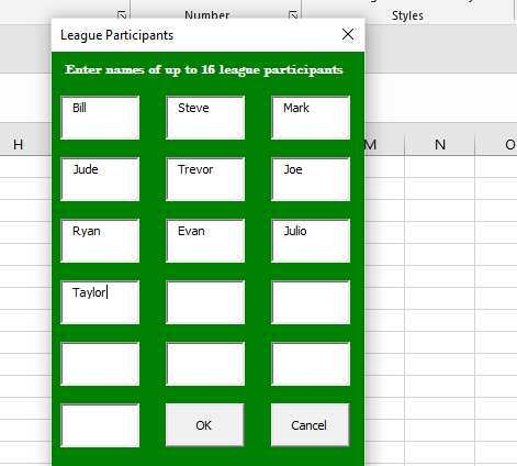
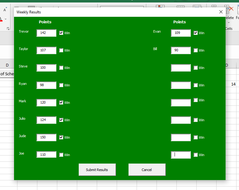
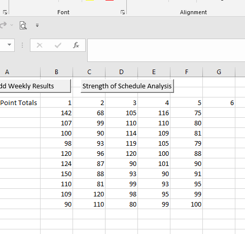
Once again, we now have a tool to help in the Poisson Binomial – Fantasy Football Strength of Schedule worksheet. To run the analysis for your league, click on the Season-long fantasy football Poisson Binomial Strength of Schedule Analysis button on the spreadsheet and enter in the names of up to 16 league participants. Then enter in your results each week and enjoy! Stay tuned next fantasy season where I will interpret the actual results of this analysis for my fantasy football leagues!
Here’s what to do:
Download the Poisson Binomial Fantasy Football SOS worksheet
Enable Macros
Choose the mode you’d like to run
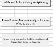
Generate a simple list of all combinations of 0 and 1 up to 20 digits long
Run a Poisson Binomial Analysis for up to 20 trials
Start a full season fantasy football Strength of Schedule analysis
Run a strength of Schedule analysis at any point in the season!
Hello Hyzermetricians, for tonight’s post I will be shining an insanely bright light on the latest video from my Instagram Live Garage Putting Series.
Alright, let’s set the stage. If you haven’t seen my live putting sessions before, most of them consist of fifty putts. Sometimes I bring in obstacles or I move the basket up onto a stair to mix things up, but for the purposes of last night’s video, I attempted 50 straightforward 19-foot putts.
I’d love to think that I should make 100% of these 19-footers, but sadly that is not (yet) the case. Instead, I hypothesized that my true putting percentage from this range was 95%. The rest of this post explains how I used my putting session last night to create a test of this hypothesis, and how you can perform a similar test too!
Suppose for a second that my hypothesis is correct, I am indeed a 95% putter from 19 ft. That doesn’t mean that I will always make 95% of my putts whenever I shoot a video. In fact, if I only attempt 50 putts at a time, it’s impossible to make exactly 95% of my putts. In some of my putting videos I’ll make more than 95% of my putts, in others I’ll make less. Given this variability, and the fact that I don’t actually know my true putting percentage, how can I ever determine if my hypothesis is accurate? Let’s find out. Roll the video!
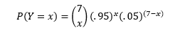
For starters, let’s look at the first seven putts from the video, of which I made five. It doesn’t take a math wizard to know that if I was truly a 95% putter like I hypothesized, 5 out of 7 (71%) is not very good. In fact, it’s probably very rare for a 95% putter to ever go less than 6 for 7! How rare? The probability of a 95% putter making Y=x putts in 7 attempts can be expressed by the below equation:
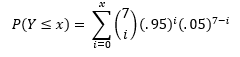
And the probability of a 95% putter making Y≤x putts in 7 attempts can be expressed by the below:
(Note, for the purposes of this exercise, I am assuming that each putt is an independent trial whose result is unaffected by any other putt in the video). If you’re wondering where these equations came from, in this exercise we are treating Y as a binomial random variable.
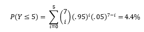
So, if I was truly a 95% putter, then the probability of me making less than or equal to 5 putts in 7 attempts is:
Remember, I want to use my putting video to test my hypothesis that I am indeed a 95% putter from 19 ft. Suppose that I create a testing procedure that says “If the observed outcome has a less than 5% chance of occurring, then reject the hypothesis.” Under this testing procedure, I would reject the hypothesis if 5 or less putts were made, but would accept the hypothesis if 6 or more were made. Thus, under this test, based on the first seven putts of my video, I’d reject the 95% hypothesis. How sad.
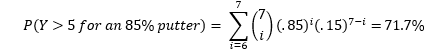
The testing procedure mentioned above has a major downfall. It had an extremely high probability of erroneously accepting the hypothesis, even if it was untrue. Suppose that my true putting percentage was 85%. Even under this lower putting percentage, it’s completely feasible that I could have made 6 or even 7 of my first 7 putts, causing us to NOT reject the hypothesis of 95%. Under the test described above, the probability of accepting the 95% hypothesis for an 85% putter is:That means that even a putter much worse than 95% could easily trick the test into accepting the 95% hypothesis. Thus, the test is not very accurate with only seven putts. We can improve upon it with more trials! Let’s look into what happened for the rest of the video.
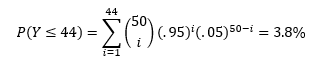
Suppose we follow the same testing procedure as we did before: “If the observed outcome has a less than 5% chance of occurring under when the existing hypothesis is true, then we reject said hypothesis.” However this time, instead of 7 putts as my sample size, I now have 50. This procedure would dictate that we reject the hypothesis for 44 or fewer made putts. Probability of observing this for a 95% putter is:In the video, I made 46 of the 50 attempts, so under this test, we would NOT reject the 95% hypothesis. Hooray! But remember the downfall of our earlier test… that test had a high probability of accepting the 95% hypothesis for significantly worse putters than 95%. To contrast, let’s see how the new testing procedure does at weeding out 85% putters:This result, compared to the 71.7% result from the initial testing procedure shows that a sample of 50 putts is far more accurate than a sample of just 7.
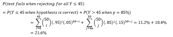
Even though the new test procedure based on 50 putts is an improvement from our earlier procedure based on 7 putts, it could be even better! Note, the probability that our test fails is equal to the sum of the two percentages in the equation above.
That’s a fairly high probability that our test will fail! If we choose to change our testing procedure so that we only reject when Y≤45, then we can improve the accuracy of the test.
Thus, a testing procedure that rejects the hypothesis for all Y≤45 has a lower probability of failure than one that rejects for all Y≤44. In fact, the Y≤45 test is the most accurate testing procedure for testing a 95% hypothesis for a sample size of 50 putts.
There’s a lot to unpack in all of the equations and commentary above. And any time the summation operator appears, especially for large numbers, the math can become super tedious. That’s why I created the Putting Hypothesis Tester for you to use in your putting practice.